

Udacity Machine Learning Nano Degree (MLND), Capstone Project, December 2018
Initial Proposal
This project will create a Convolutional Neural Network (CNN) model using supervised training to detect intruders from static images taken from an IP Camera.
Domain Background
As this is not an image classification problem (identifying one or more objects) but rather a binary determination to either produce an EMPTY or an INTRUDER image classification, this could be performed by many other types of supervised learning algorithms including decision trees, clustering, SVN or GMM. However, as my interest is in neural networks I would like to try and create a CNN network given a combination of filter sizes and layers.
Previous work done on simple or binary classification within images were done mainly with other types of algorithms, particularly SVM (link , link). Current discussions regarding neural network and security cameras focus on identifying objects and human intent in video streams (link, link, link), which is much more involved than my simple binary result from a video image. While a number of successful attempts with neural networks were made with transfer learning I don’t think it is necessary in this project as the training should be able to work at a binary classification level (though this has yet to be determined).
Problem Statement
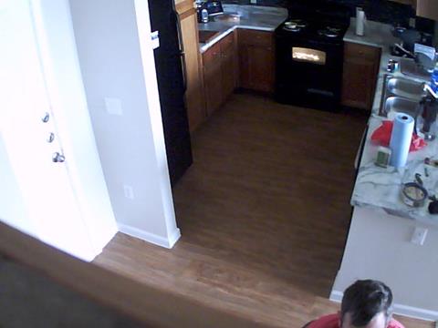
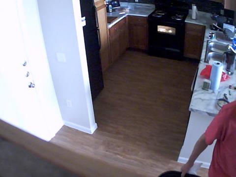
Given an image produced by an IP Camera, after training, accurately determine if there are any signs of intrusion within the photograph. In an effort to keep computational complexity lower I have define INTRUDER as anything that appears on the kitchen floor area (EMPTY is a clean kitchen floor). Of course this type of classification would not work in many homes but as a single occupant of an apartment it should be effective. Most likely the most difficult aspect of the training is that the images captured by the camera vary considerably by the time-of-day light source (natural light and/or indoor light) and in darkness when the camera switches to infra-red.
Datasets and Inputs
Images have been obtained from an older (circa 2007) Chacon IP Camera sitting on a home network. A Java routine was used to capture one image (standard definition of 640 x 480) per second for one week, producing approximate 366K images. Images have a filename with the following format:
ipcam_yyyy-mm-dd_hh.mm.ss.sss.jpg.
Solution Statement
At this point there are a number of unknowns as to how to achieve a decent CNN model. Some initial decisions will be a best guess and changes made as training session are iterated. Current questions include:
- What sampling of EMPTY images to INTRUDER images are needed (can there be a ratio or must it be balanced; assuming representation of all different light modes, but how many images of each are needed)
- How many layers will be necessary in the model
- Will ReLU be an effective activation function for this problem
- Will it be necessary to reduce RGB to grayscale at the expense of accuracy
- Will it be necessary to reduce resolution size for the mode to infer on older hardware
Benchmark Model
Standard neural network benchmark models are focused on classification (identifying objects in images). CIFAR and ImageNet are two examples that are often benchmarked for this classification. Previous work done in this area used SVM and it would be possible to find a benchmark but this would require me to code twice (once for the CNN model and once for the SVM benchmark).
Evaluation Metrics
This project will use the ROC (link) and a Logarithmic loss (log-loss) (link) for the evaluation metrics. I will use the scikit-learn Classification Report for additional analysis.
Project Design
The dataset will be supervised learning using images defined as EMPTY or INTRUDER. The current dataset is very large (17K images for INTRUDER and 340K images for EMPTY). I will be coding the project in Python 3.5 using the Keras with Tensorflow in a defined Anaconda environment. Standard public available Python libraries also to be used include: scikit-learn, numpy, opencv, pillow.
The coded routine will be iterated a number of times with adjustments to determine the best network to achieve a 95% success rate:
- Image-preprocessing
- Size reduction (if necessary, based upon performance and memory usage)
- Channel reduction (if necessary, using OpenCV)
- Image to matrix transformation
- Define epoch
- Create neural network (Keras using Tensorflow)
- Sequential model
- Image input of 640 x 480, RGB
- Filter size TBD proportional to the image size
- First layer(s) is Conv2D with ReLU
- Second layer(s) is Dense layer with 2 outputs using ReLU
- Train and validate network
- Test network
- Record accuracy rating
Analysis
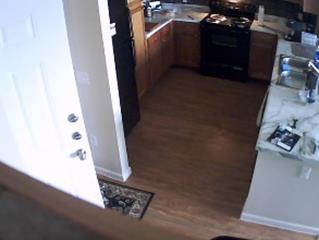
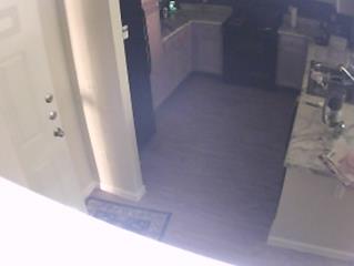
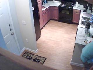
The master dataset are images (640 x 480, jpg / jpeg format, 3 channel color RGB, 35KB in size) taken from an IP Camera, approximately one image per second. The initial dataset contains 366K jpg files (for a total of 12.6 GB) from the IP Camera, starting the afternoon of June 13th and finishing on afternoon of June 18th, 2018.
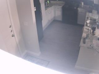
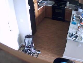
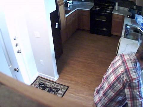
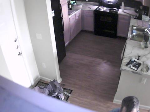
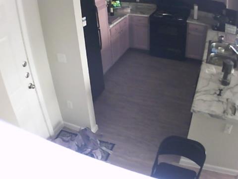
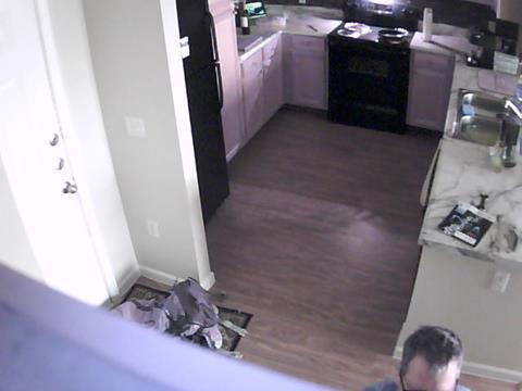
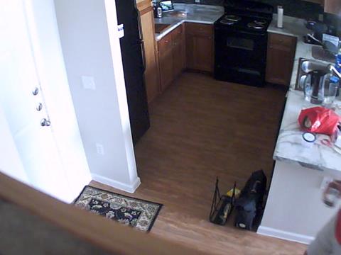
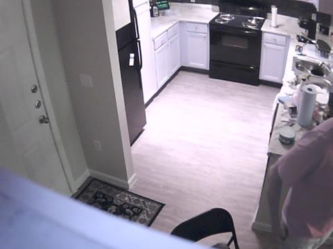
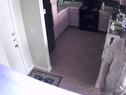
Data was hand-sorted into two categories: EMPTY and INTRUDER. EMPTY are images that contain a clean kitchen floor (no humans or artifacts on the kitchen floor). INTRUDER are all other images.
EMPTY contains the most amount of data (340K jpg images for a total of 11.7 GB) and was sorted by date into six folders based upon the date of generation. In general the middle days have more data than the start / end days (as the capture program was started in the afternoon on the first day and ended on the afternoon of the last day). In addition some days have less images than other days due to problems with the robustness of the capture program which were resolved as problems were found. On average there are 72K jpg files per day in the latter days.
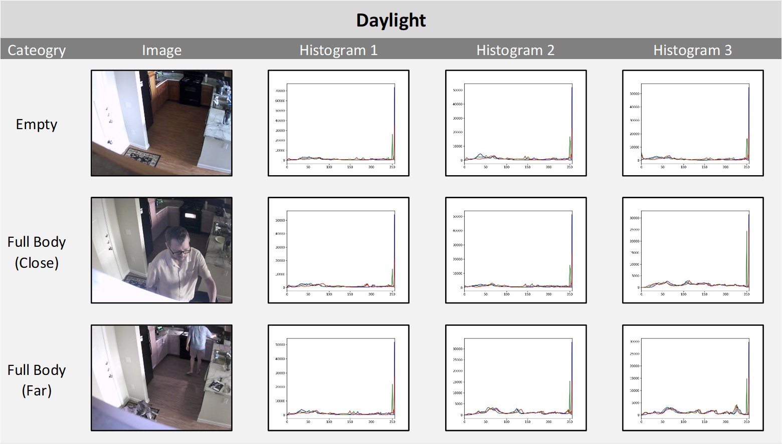
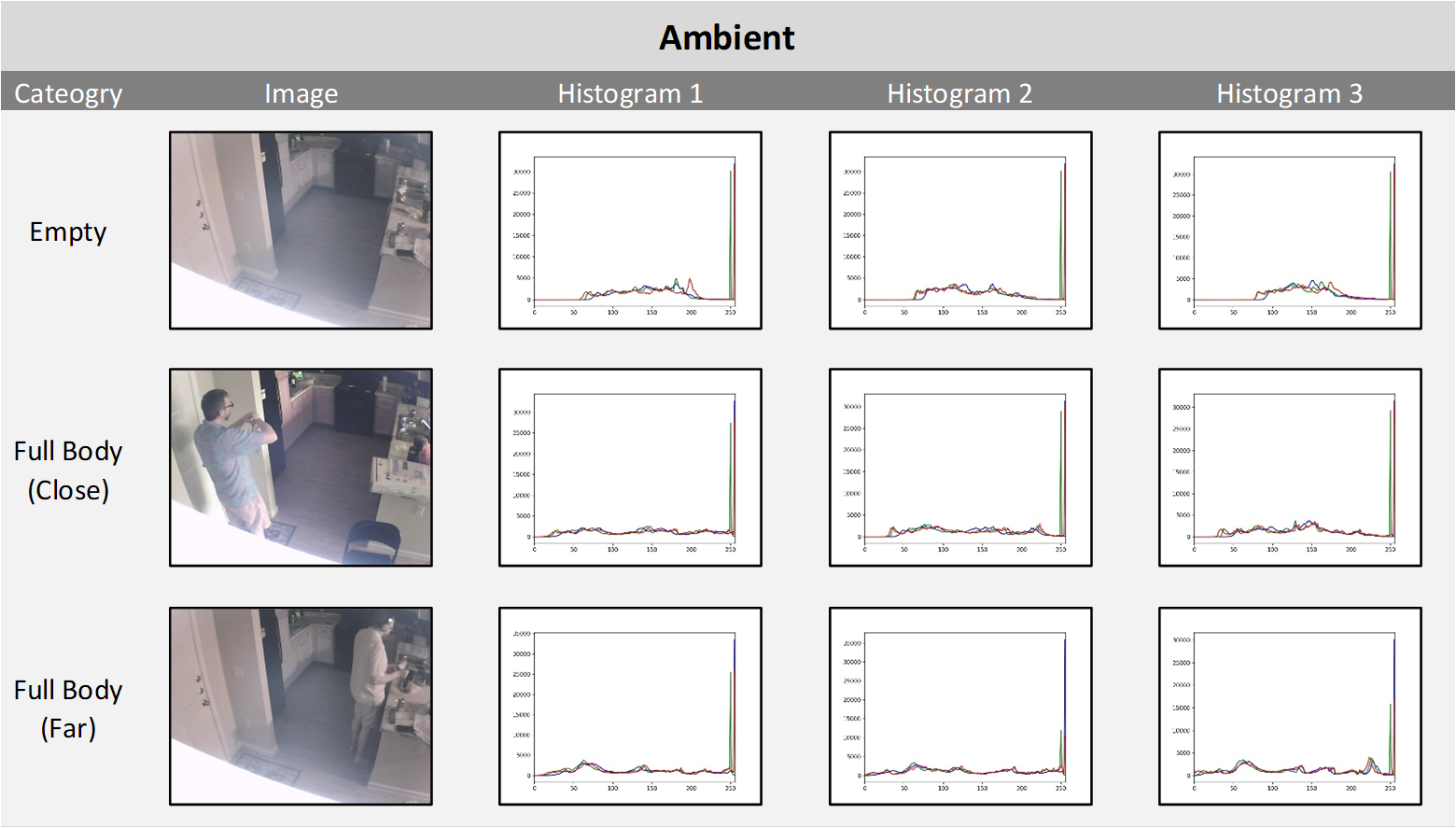
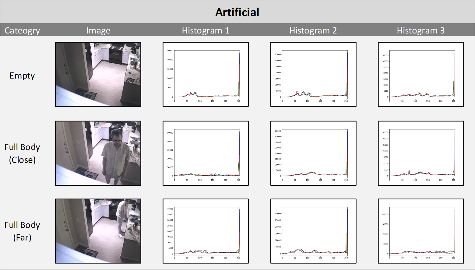
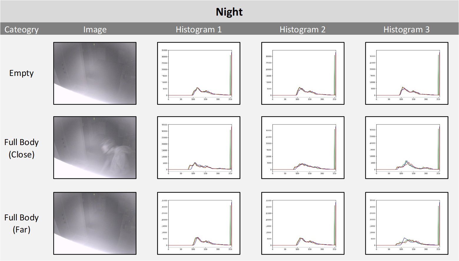
Image Light Source Histograms
Images can vary from each other in quality and features, for both EMPTY and INTRUDER, depending on the type of light:
- Daylight – natural sun light that illuminated the room from North facing windows (i.e. direct sunlight never entered the apartment)
- Ambient light – either outside evening light and/or light in other parts of the apartment
- Artificial light – direct, overhead lighting from incandescent and/or halogen lights
- Night – (no light) in which the IP camera switches to infra-red
While it is difficult to perform feature extraction from images for classification another approach is to show image tonality comparisons. Below are combined RGB intensity histograms (link) for each light category for both EMPTY and INTRUDER (Full Body Close, Full Body Far). As the images are composed of three color channels (Blue, Red, Green, or RGB) and the training is performed on RGB images without conversion to grayscale the histograms (generate_histograms.py) show the range of each channel. A random sample of three images for each light category were chosen to show the consistency of the histograms within that category. It is interesting to see that while all four light categories have very distinct histogram signatures for EMPTY images, in some cases (Ambient and Artificial) the signature changes when an INTRUDER is in the image and the histogram takes on the signature of the Daylight histogram.
Additional INTRUDER Categories
As the FULL BODY (INTRUDER Close and Far) is the substantial portion (17K images) of the non-EMPTY dataset, additional separation of the INTRUDER subset was necessary for accuracy:
- Some of the clearly needed INTRUDER images were very small in number and could easily be missed in the randomized copy program and were placed into their own folders to be copied
- The NIGHT category (as seen above) only had 223 images and the majority of them must be included in the training, test, validation and inference
- A third INTRUDER category, DOOR (122 images) showing the entry door as not closed must be included in all four phases.
|
|
- TRACES (7K images) contain INTRUDER artifacts like partial body, human shadows on wall, or a non-clean floor. It is possible that not all TRACES images may have been accurately removed from the EMPTY dataset (often the elements of human traces in the image are subtle, for instance when a human does not appear in the image but creates shadows). For this reason TRACES will not be used in the training data as it could be in conflict with the incorrectly labelled EMPTY images. However, TRACES will be used for the inference check.
|
|
|
Choosing CNN
There are two big advantages to using a CNN network on image data for this project:
- It automatically extracts out features from an image (it doesn’t require manually created filters)
- It doesn’t convert an image into a vector thus retaining the relational / compositional feature within the image
The convolutional layer is created by extracting out the greatest value from an area of the image by sliding a filter (a matrix of a certain size) over the image area and taking the greatest value via matrix dot product multiplication (link). The initial values of the filter are random and change as back propagation (link) adjusts the filter values to match the desired outcome. Adding a pooling option, in which the parameters are reduced by creating a smaller structure, creates a new feature set. Applying the convolutional layer and pooling many times enables features to emerge. Finally each layer has an activation function that determines the result output. For image classification the ReLU (Rectified Linear Unit) works well by converting all output between 0 and 1, basically forcing the answer to be positive (link). The final layer needs to use a sigmoid activation to force a binary answer.
Implementation of the IntruderNet CNN model
Subset data extraction
In trying to determine how to easily and consistently create a subset of data in an automated way, for as many times a needed, a number of factors had to be considered:
- It wasn’t clear if the CNN training would be able to use the image files in the current composition or if they would need to be transformed (or how and where that should be done)
- It wasn’t clear how many image files could be used in training in one fit statement (as opposed to batching more data); if the training was 60% of the subset total then the testing and validation should be 20% each, for a 100% of the data subset plus an additional extraction for the inferring phase
- The data subset needed to balanced (EMPTY and INTRUDER features should have the same number of images) and INTRUDER should include all of the smaller features (DOOR and NIGHT) as well
- It would be necessary to make sure that images were not duplicated in the four phases of creating and verifying the IntruderNet model (i.e. an image should only be used once). The four phases being: training, testing, validating and inferring (once the model has been trained)
A command line Java program (GetRandomFilesFromDir.java) was coded that could randomly copy or move a pre-determined number of images to a destination folder. In this way all the images needed for the entire data subset could be copied into training folder and from the training folder a percentage of data could be moved to test, validate and infer folders.
rm images/train/empty/* |
Figure 2 – From getphotos.sh, sample statements for Subset Data Creation |
The GPU server contains 32 GB of RAM. After some trial-and-error it was determined that the server could comfortably load 4,800 images before using substantial disk cache. As this server only had one disk for performance reasons it was advantageous to keep as much information in RAM as possible without having the disk intensive process of transferring data to and from RAM.
Transition to Current Training Environment
My environment setup (hardware and software) for this Capstone Project was the same setup I use for most of my development work, and all of the exercises for the Udacity Nanodegree Machine Learning. On my laptop I use a VMWare Windows 10 Pro environment with 4GB RAM. In cases where I need a more substantial RAM / CPU / disk configuration I would then transfer the source code and data to my remote server hosting VMWare Ubuntu images. The server is only accessible via a command line (SSH). For this project I built a GPU server (link) using Ubuntu 16.04 LTS; also only accessible via a very slow SSH connection.
As this Capstone Project has a large dataset and is computationally expensive to the point where a CPU in a VM environment would be inadequate, in the VM image I would create a model using PyCharm, verify that it worked against an extremely small data subset, less than 100 images and three epochs, and then move it the GPU server for training with various epochs (running from the command line). I had chosen Keras / Tensorflow as the primary method for creating a CNN model (Keras as it hides the complexity of creating a Convolutional Neural Network and sits on top of Tensorflow, and Tensorflow as it a very robust neural network framework that works with Nvidia GPU cards). In both environments (VM and GPU server) the setup leveraged Anaconda3 as it is very easy to use conda install (as it automatically installed any dependencies). Particularly the conda install was able to use CUDA 9.2 (the Nvidia required libraries to access the GPU) on Ubuntu 16.04. On the Windows VM I created a virtual conda environment TF-CPU (Tensorflow running against a CPU) and on the GPU server I created a virtual conda environment TF-GPU (to access the GPU on the server).
I was able to add a 2nd GPU to the server and take advantage of the Keras parallel_model library to access more than one GPU. This initially require two code bases, one for the CPU and one for the multi-GPU. To avoid two code bases I extracted out the CNN model into a separate file (model38.py) as the VM Python training file used the Keras model and the GPU server used the Keras Parallel Model (for multi-GPU access). Thus only the modelXX.py file had to be moved to the GPU server.
My intention was also that the model created during the training could then be moved to any Keras / Tensorflow environment (CPU, GPU or multi-GPU) however, despite much debugging and research effort in this area I have yet to resolve the issue that the multi-GPU model appears firmly associated to a multi-GPU environment and fails on all others. This appears to be a bug in Keras. Work on this in on-going. My next step is to extract out the Keras library and code the CNN in Tensorflow directly.
One consequence of my environment setup is that as my CNN development on the VMWare only used less than 100 images I was never able to determine the accuracy of the training as the dataset was too small. When I transferred the code to the GPU server, despite what type of model I created, I never achieved an accuracy rating higher than 50%. But once, after creating create more than 30 models, the GPU server had a 70% or greater accuracy. Running the Python program again then showed the accuracy was back to 50%. I was unable to determine the source of this inconsistency. It isn’t clear if this is a caching issue, a Keras or Tensorflow issue, or something else.
Out of desperation I started to use my laptop as a development machine. (I use the laptop as my primary computer for all activities with many VMWare images and as a general rule I try to keep it as a clean machine and greatly hesitate to use it for other purposes.) The laptop also has an Nvidia GPU (GTX 1050). Running the earlier models on the laptop showed that indeed the training accuracy would better than 50%. I then switched the GPU server to use a Python environment with pip3, ignoring the Anaconda3 structure. I was able to get accurate results. Luckily that solved my problem. However, this required downgrading my Ubuntu environment to CUDA 9.0 and CUDNN 9.0.
I would then use the laptop for 3 or 10 epoch training with 4,800 images (it also had 32 GB of RAM with 4 GB GPU). It would take over four minutes for epoch. The GPU server had a much faster performance with an average time of one minute per epoch. Depending on how the test accuracy of the model trained on the laptop I would then move it the GPU server for large epoch training.
Project Construction
My main coding exposure to a CNN was from working on the MLND CNN Mini-Project (aka Dog Project). It provided all of the concepts I needed to create my own CNN, providing good examples of OpenCV, Keras, sklearn.datasets, and tqdm for creating tensors, and how to create, train and infer a CNN. It wasn’t clear if extracting out the relevant coding components (the Dog Project also had face recognition, inferring against pre-trained Keras models, like using:
from keras.applications.resnet50 import ResNet50
and then applying to my larger color images (not using the cv2.cvtColor(img, cv2.COLOR_BGR2GRAY)) would have any problems, however it worked without issue.
One decision was how best to label the data that would be fed into the model. As the data was separated into their different features (EMTPY and INTRUDER) the label is derived directly from the folder names (train_intruder_multigpu-05.py), using sklearn.datasets.loadfiles (link):
def load_dataset(path): |
Two additional settings that I would perform each time I started a new Python session on the GPU server:
- As the GPU server is headless (i.e. it doesn’t have a GUI), Tensorflow at times would cause a race condition with CUDA causing the CPU to go 100% and uptime higher than 20 after finishing a training session (link). To avoid this problem the following command should be run the first time a user logs in to ensure that CUDA stays persistent:
sudo nvidia-persistenced --user aholiday - An environment variable that needs to be set when using a command line Python when the programmer wishes to use Python files in other folders is to point Python to the location of these folders:
export PYTHONPATH=./models_intruderNet
Program Composition
At a high level the train_intruder_multigpu-05.py (the code that trains the CNN) can be divided into four sections:
- Load the image file names and their labels
|
|
- From the file names, load images and then convert to an array (each pixel in a range of 0 to 255) then divide each pixel to normalize all data to 0 -> 1
|
|
- Load the model (in this case
model38.pydefined in theimportstatement) and train (usingmodel.fit) using the data
|
|
- Load the best model and show the statistics
|
|
Benchmarking
In an attempt to benchmark my results I created both AlexNet and VGG16 networks. However they were very heavy in parameters and it would have been necessary for me to reduce my image size in order to train on my hardware. A number of models exists in the master_model.zip from the Tensorflow GitHub. These also required me to transform my images to a smaller dimension. As I had achieved high test accuracy with my current IntruderNet, and assuming that I was not overfitting the data, I consider this to be comparable to any other benchmark.
Creating the IntruderNet Model
Over a two month period I iterated through 50+ model creations to achieve a high accuracy rate. As I wasn’t sure of what type of structure would be needed in creating the IntruderNet network I initially started with a Keras Dense network (a multi-perceptron network). I then switch to a CNN network (Keras Conv2D), trying different combinations of layers, kernels and filters. Reviewing other CNN images classification networks I then added a number of Dense layers to my CNN layers.
From my manual image analysis I felt that as there were situations in which the INTRUDER in the image could be very small I wanted to make sure that I avoided loosing this information by either reducing the resolution or by reducing the complexity of the CNN. A decision was made to import that image into the CNN without any modification (620 x 480, 3 channel RGB). Another decision is that, once I realized that using only Keras Dense layers were ineffective for test accuracy, I would add a Conv2D layer to build bigger features from the previous layer. This meant starting with many small filters and gradually increasing the size of the filter for each layer.
The two primary adjustments involved the Keras Conv2D filter and kernel_size arguments. By initially keeping the filter size small the complexity of the features found would be small. Gradually increasing the filter size for each layer would increase the number of features. Keeping the kernel_size to a small number of 2 (and later layers using 3) produces a 2 x 2 sliding matrix (or grid) over the image.
I assumed that if there was no accuracy improvement within the first three epochs that I was on the wrong path. I did not try larger epochs until I was somewhat confident that I had a decent, working model. As I performed my testing it became apparent that a balance exists between a number of factors that need to work within the CPU and GPU RAM requirements:
- The size of the image
- The number of images
- The number of layers
- The methods used to reduce the parameters (thus the size within RAM) such pooling, dropouts, or flattening
My initial network only used multi-perceptrons and never achieved a result better than random (test accuracy of 50%).
model.add(Conv2D(filters=4, kernel_size=5, padding='same', activation='relu', input_shape=(640,480, 3))) |
I initially, mistakenly, assumed that if I created a large multi-perceptron without dropping any information that my accuracy would be high. Accuracy never improved despite the number of Dense layers I added.
I then started using CNN layers finishing with Dense layers (as a number of networks used this as well), but failed to use any pooling, thinking, again mistakenly, that I wanted to not lose any information and doing so would help in my accuracy.
|
|
I then started to use MaxPooling with multi Conv2D layers, as many of the networks I was researching also used this. Having at least four layers with a final GlobalAveragePooling before using a Dense network was the key to increasing my accuracy. By chance I discovered that I had a problem with my GPU server (see Transition to Current Training Environment above), getting accuracy of 74% the first time and 50% a later time (see the Transition to Current Training Environment above as to how I fixed this problem).
|
|
At this point it was just a matter of adding layers (both Conv2D and Dense) and changing the filters arguments and determine if Dropouts (to reduce the number of parameters and reduce overfitting) and were better than Pooling (to reduce the number of parameters).
|
|
I determined that for my network Dropouts worked better with the Dense layers.
|
|
Final CNN Model
The final CNN model is composed of 12 layers. The first seven layers use the Keras Conv2D (a two dimensional convolutional layer, which is effective for two dimensional images) with MaxPooling. The final five layers use the Keras Dense layers (equivalent to creating a multi-perceptron layer in which everyone node is connected to each other) with dropouts to prevent overfitting.
|
|
| Figure 3 – IntruderNet CNN Model |
The size of the CNN model became limited by the number of total parameters that can be handled in memory, in this case 3M parameters is the limit of the current environment.
__________________________________________________________________________________________________ |
| Figure 4 – IntruderNet Model Summary |
The model is the compiled with Adam and Binary Cross Entropy (model38.py).
def get_model_compiled_multi_gpu(self): |
| Figure 5 – IntruderNet Model Compile Settings |
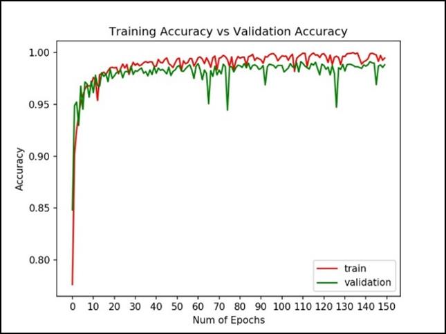
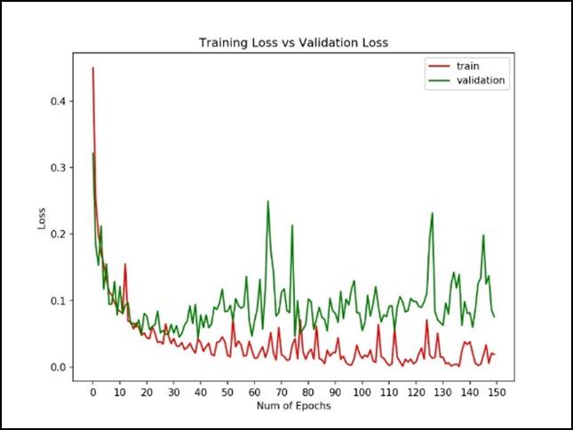
An epoch of 150 was chosen. However the best accuracy was reached at epoch 40 and all subsequent epochs did not show any improvement.
4800/4806 [============================>.] - ETA: 0s - loss: 0.0426 - acc: 0.9867 |
| Figure 6 – Peak accuracy appeared in Epoch 40 |
Results
The final model has a test accuracy result of 98.25%.
Epoch 00150: val_loss did not improve from 0.04295 |
| Figure 7 – IntruderNet Test Accuracy 98.25% |
However, the accuracy range is variable upon the data used. If the data subset used for training was scrubbed and again randomly generated from the master data source the test accuracy would occasionally reach the 99% range.
Training Results
Training vs Validation
|
|
Confusion Matrix
| Actual Class | |||
|---|---|---|---|
| EMPTY | INTRUDER | ||
| Predicted Class | EMPTY | 791 | 9 |
| INTRUDER | 19 | 781 | |
| Figure 10 – Confusion Matrix | |||
Classification Report
Classification Report |
| Figure 11 – Classification Report |
ROC
The ROC (Receiver Operating Characteristics)
ROC - Receiver Operating Characteristic |
| Figure 12 – ROC |
Inference Testing
Some additional accuracy checks were performed by inferring additional images (infer_intruderNet-03.py). The inferring was performed using 1000 EMPTY and 1000 INTRUDER unique images. From the outset it wasn’t clear how well the NIGHT (223 images) and DOOR (122 images) were integrated into the model as they were less than 0.05% of the total training data. In addition, as the TRACES images were not used in training and it wasn’t clear if they would be successfully determine to be in the INTRUDER category as at times there were only subtle indicators to suggest an intruder.
model: mod38_multi_5.i150.hdf5 |
| Figure 13 – Inference Results |
As expected for inference on EMPTY and FULL BODY INTRUDER images (which are the majority of the INTRUDER images trained), there is a very high success rate, 98%, on these images against the trained model.
The NIGHT and DOOR images (223 and 123 images respectively out of the 4806 total INTRUDER images trained) has high but not excellent results (87% inference accuracy for NIGHT and 95% for DOOR).
The TRACE images have an inference rate of 79%. While the TRACES inference results are considerably poor, for the purpose of the identifying an INTRUDER they would be supplemental to the FULL BODY training and not necessary to be relied upon for true INTRUDER detection. In the apartment floorplan an intruder would always need to enter from front door on the left (there is no other entrance) and move across the camera field. Thus FULL BODY images would be captured and trigger and alert to the home owner.
Looking closer at the TRACES results, taking the first 10 images processed shows that not training on these images gave unpredictable results.
The first 10 images inferred:
./images/infer/intruder_traces |
All inferred results should be “1”:
[1, 0, 1, 1, 0, 0, 0, 1, 1, 0, |
Accurately categorized (traces of INTRUDER)
|
|
|

|
|
Inaccurately categorized (traces of INTRUDER)
|
|
|
|
|
Conclusions
Overall the IntruderNet model achieved the ability to determine if an INTRUDER has appeared with in a certain area of the image. The CNN worked very well in defining the difference between EMPTY and INTRUDER.
The IntuderNet model works well with large images (640 x 480, 3 changes: RGB) from the IP camera and did not require any manipulation of the image (reduction in size, reduction in changes, convert to high contrast images). In addition it wasn’t necessary to train more than 4,800 images, so it was not necessary to split a large amount of images into training batches.
The lack of NIGHT and DOOR images could be problematic as the provided dataset for these features were so small. A goal should be to have NIGHT and DOOR reach the same level of inference percentage as EMPTY and FULL BODY.
Process Recap
The process I had proposed in the Capstone Proposal worked fairly well. As the programming side (data subset extraction and training) was fairly low (less than 1000 lines of code) the majority of the effort was spent trying to understand how the Keras Conv2D input arguments effected accuracy, how many layers and types of layers were needed, and debugging my testing environment to obtain consistent results.
One mistake I made is that all of the early evaluations I performed in creating the network used a categorical_crossentropy with two categories in the model:
model.compile(optimizer='adam', loss='categorical_crossentropy', metrics=['accuracy'])
and later switched to binary_crossentropy. Another tuning feature that I was unable to determine if it improved or worsen my results was using an adam vs rmsprop optimizer. I also varied the filter sizes to see if larger filters in the first layers would improve accuracy. They did not.
A major failure in this project was my inconsistent recording of results (not all results were copied / pasted into the spreadsheet and going back over how I advanced in the IntruderNet model was difficult to recreate for this report). It would be better to automatically output results into a unique file that was timestamped.
A major drawback to this supervised approach was the necessity of hand-sorting images. A very time consuming and redundant process. It would probably be easy to programmatically extract out a few images that represent the majority of the EMPTY and INTRUDER, ask the user to confirm a few of these images, and then automatically label the similar ones.
I had some difficulty in finding a CNN feature visualization coding example that could show how to show each layer feature visually. A first test was performed using pytorch but as these are manual filters it is not the same as the automatic filters that a convolutional layer would produce. As there were not any examples to use from any of the exercises from the MLND classes, this requires additional research. Some possible directions have been described in IEEE articles. A great article that tackles this problem with pointers to possible visualization libraries is: https://arxiv.org/ftp/arxiv/papers/1804/1804.02527.pdf.
Final Thoughts
Current state-of-the-art intrusion detection systems monitor video feeds in real time. It seems a one image per second timeframe (as opposed to 30 frames per second in a moving image) is an effective alternative for low cost hardware (though the training would need a more powerful server).
README for setting up a Python training environment
Environments
Two environments were used to produce the IntruderNet. A primary development environment to test to code and debug, and a training environment to perform the training and inference. The Python and Java files can be run in both environment, it is just faster on the GPU server for training (approximately one minute per epoch vs four minutes per epoch on the development laptop).
| Primary development environment |
Dell XPS Laptop |
| Training Environment |
GPU server |